Modelling of Pressurised Pipes within InfoWorks ICM

Innovyze Howbery Park Wallingford Oxfordshire OX10 8BA United Kingdom +44 (01491 821400 support@innovyze.com www.innovyze.com
Technical Paper February 2013

1. Introduction

Correctly modelling pressurised pipes, variously described as forcemains or rising mains, can be one of the more difficult aspects of the model build process.

The fundamental problem is that no equations have yet been developed which adequately represent the transition from free surface flow, such as exists in open channel or pipes which are not completely full, to pressurised flow which exists in pipes which are completely full. Pressurised flow can exist either intermittently, for example in storm pipes which become surcharged during rainfall, or permanently, for example in pumped systems or siphons.

Pipes which are predominantly free surface and only rarely surcharged are modelled using the Preissmann Slot approximation. This uses a narrow slot, which runs the length of the conduit and extends vertically up to infinity. The width of this slot can be edited, but by default is 2% of the pipe width. It is crudely shown in Figure 1.

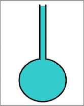
Figure 1: Preissmann slot

The Preissmann slot allows a free surface to be maintained and therefore a transition does not occur. The slot makes pipes slightly larger than in reality. This is usually compensated for by the base flow depth, which makes the pipes slightly smaller and by manually decreasing the size of the manholes, using the storage compensation feature, so that the correct volume of the below ground system is represented.

The Preissmann slot is not recommended in pipes which are permanently or very heavily surcharged (i.e. highly pressurised) for two main reasons:

1. The flow attenuation is over predicted because in a forcemain, virtually as soon as flow is introduced at one end, it will exit at the other, whereas in an open channel there would be a much longer delay in time of travel.

2. The pipe area is significantly increased and therefore the flow velocity significantly decreased. This means that the headlosses associated with pipe roughness and minor losses such as bends and junctions, which are all a function of velocity, are under predicted. This is particularly important at pumps, where the head in the head / discharge relationship is defined by both the vertical distance the water must be raised and the additional head required to overcome the losses in the forcemain. This is shown in Figure 2.

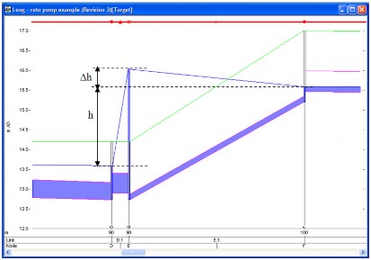
Figure 2: Head through which pumped flow must be raised

Therefore a dedicated pressurised pipe model must be used, which does not include the Preissmann Slot or base flow, approximations. There are two options for doing this, the ‘Pressure’ or ‘ForceMain’ solution models, both specified as part of the conduit information.

2. When to use pressure or forcemain solutions

The difference between the pressure and forcemains models is that in the forcemain model a minimum water level equal to the pipe soffit is imposed on the flow. No such limitation is placed on the pressurised model. The forcemain minimum level is applied to overcome two limitations of the pressure model.

The first limitation of the pressure model is that at the top (most downstream end) of a forcemain the water may not reach the pipe soffit. This is shown in Figure 3.

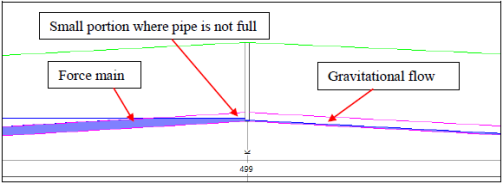
Figure 3: Top of rising main with pressure model

Due to this small portion of non-pressurised pipe, the pipe cannot be considered full all the time and therefore the pressure model is abandoned for the rest of the simulation and the equation system reverts to the Preissmann Slot approximation. In the past, several workarounds to this have been suggested such as the use of weirs and also lowering of the pressurised pipe, to ensure it is always full.

The second limitation has been observed in very long rising mains which experience relatively low levels of surcharge. Here an effect similar to water hammer, a shock wave, has caused pipes to drop out of surcharge for a fraction of a timestep. This is enough to cause the pressurised pipe model to once again be abandoned.

Note that if the pressure model is abandoned, for any reason, a warning will be given in the results.log file.

For these two reasons the forcemain solution is recommended in preference to the pressure solution.

3. An example of the forcemain solution

Figure 4 shows a fairly complex forcemain example. Nodes A to C and the pipes associated with them represent a gravity system draining down to a pumping station. Node D is the pumping station wet well which pumps forward to node F. There is an emergency overflow to node E. Node F down to the outfall at node L represents the forcemain traversing a series of hills with all pipes using the forcemain solution and all nodes specified as break nodes. This arrangement is complex to model because pressurised pipes which flow downhill are in danger of not remaining full throughout the simulation.

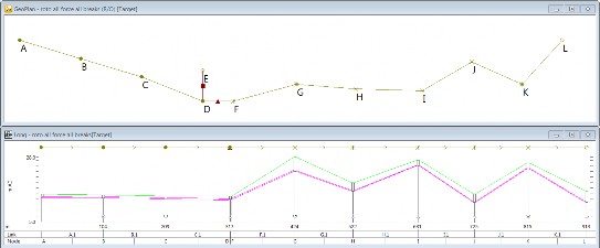
Figure 4: Forcemain example

Figure 5 shows the hydraulic profile when the pump is running.

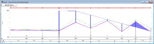
Figure 5: Forcemain in operation

Note the hydraulic profile at node K. Here the hydraulic grade line is well below the pipe level. This part of the system is acting as a siphon.

An alternative method of modelling this system is to remove the siphoning effect. This is achieved by representing the manhole at the top of each hill (nodes G, I and K) as a sealed manhole rather than break nodes.

Figure 6 shows the hydraulic profile for this configuration, measured at the same point in the simulation.

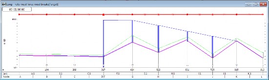
Figure 6: Forcemain without siphoning effect

It can be seen that the hydraulic grade line in Figure 6 is greater than in Figure 5. This is because the water has to be pumped up and over the hills without assistance from the siphoning effect.

Introducing sealed manholes is the equivalent to introducing air valves in to the system.

This type of representation can experience problems during initialisation. There are two changes which are often required:

The pipe immediately upstream of the outfall, in this example link K.1 is acting as a gravity pipe and should therefore be modelled with the ‘full’ solution.

Pipes in the middle of the forcemain, which are sloping downhill, such as G.1 and I.1, may cause problems with the simulation engine, relating to whether they are surcharged. This could result in the model failing to initialise and also in a generation of flow (i.e. a greater outflow than inflow reporting in the results .prn file.) It is sometimes necessary to drop the upstream end slightly so that they remain full (i.e such that the soffit of the downstream pipe is below the invert of the upstream.) Careful examination of Figure 6 shows that this has been done to Link I.1.

4. Result comparisons

Figure 7 shows a comparison of the flow in the pump (link D.1) with the flow at the downstream end of the forcemain (link K.1) for the siphoning effect shown in Figure 5.

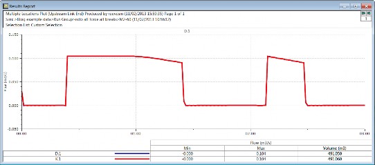
Figure 7: Forcemain flow results

The main thing to notice about the plots is that they are virtually identical, there is no attenuation along the forcemain.

Figure 8 shows the same comparison of pump and forcemain flows for the example shown in Figure 6, where air valves have been included.

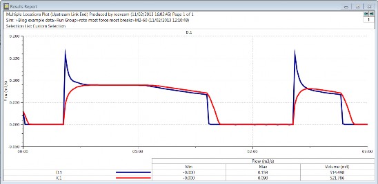
Figure 8: Forcemain flow results, air valves included

Comparison with Figure 7 shows that the pump characteristics have changed significantly and there is now significant attenuation along the forcemain. Figure 8 also shows that there is slightly more flow at the downstream end of the forcemain than through the pump. This is because levels are slightly lower at the end of the simulation than at the start. It is not something to be concerned about.

5. General points to note

The following provides a summary of good practice when modelling forcemains.

• The principles described here can also be applied to multiple pumps and multiple forcemains, including connections within the forcemain.
• The connection between the pump and forcemain downstream should always be a break node.
• Junctions, changes in gradient, changes in size and other break points should be modelled with a break node, in which case a siphoning effect will be introduced.
• Sealed manholes should be used to represent air valves, which introduce attenuation and remove the siphoning effect.
• The tick box ‘drop inertia in pressure pipes’ in the simulation parameters should always be ticked.
• Pressure pipes with a positive gradient (i.e. sloping downhill in the direction of pumped flow) represent the greatest challenge in forcemain modelling.
• Check the results .prn file for a net generation of flow, particularly when the last pipe before an outfall is a postive gradient forcemain solution.
• Initialisation problems can often be resolved by lowered the inverts of positive gradient forcemains.
• Only the ‘fixed’ or ‘none’ headloss types should be used in pressurised pipes
• Some dry weather flow should be applied upstream of the pump, even for purely storm systems, to ensure that the force main initialises full.