Representation of Culverts in InfoWorks
|
Innovyze Howbery Park Wallingford Oxfordshire OX10 8BA United Kingdom +44 (01491 821400 |
|
||
|
Technical Paper June 2011 |
|||

1. Introduction
This report describes culvert inlets and outlets as implemented in InfoWorks ICM. The representation of these structures is based heavily on CIRIA report CP/40 (Reference 1) and Normann (Reference 2).
Chapter 1 provides an overview of culvert representation, Chapter 2 presents the various flow conditions and the equations used to calculate headloss in each case. Chapter 3 provides worked examples to demonstrate each case
A culvert is typically used to route flow underneath a structure such as a major road, it usually consists of a an inlet structure to 'funnel' the flow into a concrete channel and then out via a similar outlet structure. Several examples and photographs of culverts are presented in Reference 1.

Figure 1 Schematic Long Section (Profile) of a Culvert
The culvert must be correctly modelled to accurately represent the headlosses which occur in the three elements of the culvert:
- The culvert inlet
- The culvert itself
- The culvert outlet
CIRIA (Ref 1, pg 23-25) describes six different flow conditions which dictate how the headlosses should be calculated. In each of the six cases the culvert is said to be either inlet or outlet controlled. In other words, are the headlosses through the culvert dominated by the headlosses at the inlet (inlet controlled) or at the outlet (outlet controlled)? This rather complex set of scenarios is further complicated because whether the culvert is inlet or outlet controlled only affects the inlet calculations. Under all conditions the operation of the culvert itself and the culvert outlet is governed by the same set of equations.
2. Flow Calculation
2.1 The Inlet
The six scenarios presented in Reference 1 can be reduced to three modes, as presented below.
- The flow at the upstream end of the culvert is super-critical and the culvert is un-submerged, presented in Chapter 2.1.1.
- The flow at the upstream end of the culvert is super-critical and the culvert is submerged, presented in Chapter 2.1.2.
- The flow at the upstream end of the culvert is sub-critical, presented in Chapter 2.1.3.
Whether the culvert is super or sub-critical, is dependent on the Froude number.
Fr > 1 then super-critical
Fr < 1 then sub-critical
|
|
Fr = Froude number v = Velocity g = 9.81 m/s2 h = Depth |

Whether the inlet is submerged or un-submerged does not simply depend on if the water level exceeds the soffit of the culvert, it depends on the discharge intensity according to CIRIA (Ref 1 pg 133).
|
|
DI = discharge intensity Q = design discharge (m3/s) A = culvert area (m2) D = culvert height (m) |

- If DI < 3.5 then the culvert is un-submerged.
- If DI > 4.0 then the culvert is submerged.
- If DI is between 3.5 and 4.0, it is in a transition zone where there is linear interpolation between the two equations, based on the larger of the flows.
It is possible to tell which mode a culvert is operating in, by tabulating or graphing its 'status'. This option is only available if the Timestep Log box is ticked when the simulation is scheduled. This box is located under 'Diagnostics' in the Run dialog. Table 1 presents the status number corresponding to each flow condition.
| Condition | Status Value |
|---|---|
| Super-critical and un-submerged | 1 |
| Super-critical and submerged | 5 |
| Super-critical and transition | 33 |
| Sub-critical | 9 |
| Sub-critical, linearised | 25 |
| Reverse flow | 3 |
| Inactive | 0 |
2.1.1 Super Critical and Un-submerged
In this case the flow at the upstream end of the culvert (immediately downstream of the inlet) is super-critical, Froude number greater than 1.0, and the discharge intensity is less than 3.5.
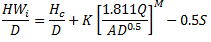
Depending on the type of inlet structure, as defined in CIRIA (Ref 1 Table D1, pg 151) either of two equations A and B can be used to calculate the water level immediately upstream of the inlet. Both equations are presented in CIRIA (Ref 1 pg 134.)
Equation A:
|
|
HWi = water depth at the inlet (m) K,M = constants taken from CIRIA (Ref 1 Table D1, pg 151) S = culvert slope
yc = critical depth (m) vc = critical velocity
To find yc and vc, solve the equation below for Ac.
Ac = area of flow at critical depth (m2) T = culvert width (m) |


Equation B:
|
|
|

2.1.2 Super-critical and Submerged
In this case the flow in the channel is super-critical, Froude number greater than 1.0, and the discharge intensity is greater than 4.0.
Here the water depth at the inlet is calculated from the equation.
|
|
c, Y = constants taken from CIRIA (Ref 1 Table D1, pg 151) |

2.1.3 Sub-critical
The flow in the channel is sub-critical, Froude number less than 1.0.
In this situation the relevant equation 5, 6 or 7 above can be superceded by equation 8 below, if it provides a higher water level in the channel immediately upstream of the culvert inlet.
|
|
hi = headloss across inlet Ki = constant taken from CIRIA (Ref 1) (Table D1, pg 151) Vb = velocity in the culvert |

Equation 8 is presented in CIRIA (Ref1 pg 141):
Note that there are discrepancies between the K, M, c and Y constants quoted in References 1 and 2.
2.2 Culvert Headloss
The culvert itself covers three elements of headloss.
- Headloss due to trash screens (CIRIA Ref 1 pg 137)
- Headloss due to bends (CIRIA Ref 1 pg 141)
- Headloss due to friction (CIRIA Ref 1 pg 143)
Headloss due to friction is represented by specifying a channel roughness (Manning or Colebrook White) for the culvert.
The headloss due to trash screens and bends is represented by calculating a fixed headloss coefficient K and applying it to the upstream end of the culvert.
K is calculated by solving the equation:
|
|
hs = headloss due to trash screens hb = headloss due to bends
Ks = screen coefficient (assumed to be 1.5 from (CIRIA Ref 1 pg 139)) Vs = velocity between the trash screen bars, simply calculated from the 'total bar area' in the upstream channel VUC = velocity in the upstream channel
Kb = bend coefficient, taken from (CIRIA Ref 1 Design Chart D5 Appendix A1) |


The downstream end of the culvert is specified with a headloss of 'none'.
2.3 Outlet Headloss
Regardless of the flow conditions, the headloss in the outlet is calculated from the equation:
|
|
Ko = outlet headloss coefficient, usually 1.0 (CIRIA Ref 1, pg 141) Vb = velocity in the culvert Vdc = velocity in channel immediately downstream of the culvert |

3. Worked Examples
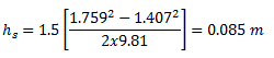
A typical culvert arrangement is presented in Figure 2 below.

Figure 2 Representation of a Culvert
A.1 is the upstream channel, B.1 is the culvert inlet, C.1 is the culvert itself, D.1 is the culvert outlet, E.1 is the downstream channel and F.1 is a weir, which is simply applied in order to raise the downstream water level and is not usually required in culvert design (in this analysis it is not used at all.)
All coefficients must be specified even if the flow conditions mean that they will not be used.
This Chapter presents the following examples:
- Chapter 3.1, super-critical and un-submerged, using Equation A. In this example the full calculations are completed for the inlet, the culvert itself and the outlet. In the remaining examples only the method of calculation for the headloss in the inlet changes and therefore it is only the inlet calculations that are presented.
- Chapter 3.2, super-critical and un-submerged, using Equation B.
- Chapter 3.3, super-critical and submerged.
- Chapter 3.4, sub-critical flow, but inlet conditions (equations 5, 6 or 7) dominate.
- Chapter 3.5, sub-critical flow, but outlet conditions (equation 8) dominates.
3.1 Super-critical and Un-submerged, Equation A
This example uses the network shown in Figure 2 and a constant inflow of 6.4 m3/s.
The results are presented in Figure 3.

Figure 3 Super-critical, un-submerged, Equation A
3.1.1 Inlet Headloss Calculations
Calculate the Froude number, from equation 1:
|
|
> 1, therefore super-critical |
|

Calculate discharge intensity from equation 2:
|
|
< 3.5, therefore un-submerged |
|

The culvert inlet has a stats of 1, which matches the condition presented in Table 1.
Assume that the inlet is 90 and 15 degree rectangular concrete wingwalls. The coefficients to be used are presented in Figure 2.
From equation 5:
|
|
therefore Ac = 2.15 |
|
|
therefore yc = 2.15/2.4 = 0.898 m vc = 6.4/2.15 = 2.976 m/s |
|
|

From equation 4:
|
|
|

From equation 3:
|
|
|
|
Therefore HWi = 1.516 m.
From Figure 3 it can be seen that the water depth at the downstream end of the channel (link A.1) is 1.516 m.
3.1.2 Culvert Headloss Calculations
To solve equation 11:
From Figure 3 it can be seen that Vuc = 1.407 m/s.
Assume that the bars cover 20% of the available area, therefore:
|
VS = 1.407 / 0.8 = 1.759 |
|
|
|
|
|
|
Taking a value of kb of 0.214 from Design Chart D5 of CIRIA (Ref 1) and solving equation 12, gives a value of hb = 0.213m
Therefore from equation 10, hT = 0.213 + 0.085 = 0.298 m.
Solving for K in equation 9 gives:
|
|
|
|

Therefore K = 0.3, which is applied to the upstream end of the culvert as shown in Figure 2.
The results in Figure 3 show that the depth at the upstream end of the culvert (link C.1) is 0.574 m. The culvert invert level is 25.80 m. Therefore the water level at the upstream end of the culvert = 26.374 m. From Figure 3 it can also be seen that the water level in the manhole immediately upstream of the culvert (node C) is 26.704. Therefore the headloss calculated by InfoWorks is 26.704 – 26.374 = 0.330 m.
From the standard head loss equation 9:
|
|
|
|

This matches the model results.
3.1.3 Culvert Outlet Headloss Calculations
Solving equation 13, using the value of Ko=1.0 (as shown in Figure 2) and the values of Vband Vdc shown in Figure 3, gives:
|
|
|
|

From Figure 3 it can be seen that the depth in the downstream end of the culvert is 1.216 m and the depth in the upstream end of the channel is 1.147 m. Therefore the headloss across the culvert outlet is 0.069 m, which matches the manual calculations.
3.2 Super-critical and un-submerged, Equation B
In this example only the inlet calculations are presented as the culvert and outlet are the same as presented in Chapter 3.1.
This example uses the networks shown in Figure 2 and a constant inflow of 6.4 m3/s. Values of K = 0.515 and M = 0.667 are used, which are consistent with Table D.1 of Reference 1.
The results are presented in Figure 4.
Figure 4 Super-critical, un-submerged, Equation B
|
|
|
|

From Figure 4 it can be seen that the depth at the downstream end of the channel (link A.1) is 1.472 m.
3.3 Super-critical and Submerged
Here only the inlet calculations are shown, because as mentioned previously, the headloss in the culvert itself and the outlet are calculated by the same method as the un-submerged condition. This example uses the same culvert arrangement as shown in Figure 2, except the height fo the culvert is reduced from 2.4 to 1.0 m. Therefore from equation 2:
|
|
> 4.0, therefore submerged |
|

Therefore from equation 7 and Figure 2:
|
|
|
|

HWi = 1.728 m
From Figure 5 it can be seen that the status of the culvert inlet is 5, matching the condition presented in Table 1. The depth at the downstream end of the channel predicted by the model is 1.728 m, this matches the manual calculations.

Figure 5 Super-critical Submerged Condition
3.4 Sub-critical (Equation 5 dominating)
In sub-critical flow, the upstream water level is defined by the maximum of either the inlet (equation 5) or outlet (equation 8) conditions.
In this example, again only the inlet calculations are provided, as the methodology for the culvert itself and the outlet are unaffected. This calculation uses the same culvert arrangement as shown in Figure 2, except the downstream end of the culvert, culvert outlet and downstream channel are raised from 24.8 to 25.7, effectively reducing the culvert slope from 0.01 to 0.001. The upstream headloss for the culvert (link C.1) is set to 0.9.
The results of this simulation are presented in Figure 6.

Figure 6 Sub-critical Condition Inlet Control Dominating
From equation 1:
|
|
therefore sub-critical |
|

Therefore either inlet or outlet control will dominate, based on whichever gives the greatest depth.
Inlet control
From equation 3:
|
|
|
|

HWi = 1.527
Outlet control
From equation 9:
|
|
|
|

Therefore level at upstream end of culvert (node C) equals:
Invert + upstream depth + headloss = 25.8+1.21+0.223 = 27.233 m, which matches the result presented in Figure 6.
Therefore the velocity at the downstream end of the inlet equals:
Q/A = 6.4/(1.21 + 0.223)*2.4 = 1.86 m/s
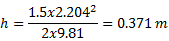
Therefore, from equation 8:
|
|
|
|

Therefore HWo = 1.21 + 0.223 + 0.088 = 1.521 m
HWi > HWo and thefore HWi dominates
The HWi value of 1.527 m matches the upstream depth of link B.1 presented in Figure 6.
Note that the culvert inlet status is defined as 1.0, which from Table 1 corresponds to a super-critical and un-submerged condition. This is an indication that the inlet control equation is dominating, as it would under such flow conditions.
3.5 Sub-critical (Equation 8 dominating)
This example matches that presented in Chapter 3.4 except the headloss at the upstream end of the culvert (link C.1) is increased from 0.9 to 1.5. The results are presented in Figure 7.
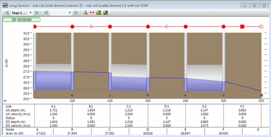
Figure 7 Sub-critical Condition Outlet Control Dominating
The calculation of HWi is unaffected, remaining at 1.527 m.
Outlet control
From equation 9:
|
|
|
|
Therefore level at upstream end of culvert (node C) equals:
Invert + upstream depth + headloss = 25.8 + 1.21 + 0.371 = 27.381 m, which matches the result presented in Figure 7.
Therefore the velocity at the downstream end of the inlet equals:
Q/A = 6.4/(1.21 + 0.371)*2.4 = 1.687 m/s
Therefore, from equation 8:
|
|
|
|

Therefore HWo = 1.21 + 0.371 + 0.073 = 1.654 m
Now HWo > HWi and therefore HWo dominates.
The value of HWo matches the upstream depth in the inlet (link B.1) presented in Figure 7.
Note that the status of the culvert inlet is now 9.
References
1. D Ramsbottom, R May and C Rickard. Hydraulic Design of Culverts, CIRIA Funders Report CP/40, November 1996.
2. Jerome M Normann, Robert J Houghtalen and William J Johnston. Hydraulic Design of Culverts, Report No. FHWA-NH1-01-020 HDS 5.
Article © Innovyze 2011