Network Model

The network model is used to generate the concentration of dissolved pollutants and suspended sediment at the nodes.

In InfoWorks ICM, the urban drainage network is made up of nodes and links. Nodes are used to model storage volume in the network and may be points at which conduits meet. Nodes may, for example, represent:

• manholes
• outfalls
• tanks
• pump wet-wells
• ponds

The governing equation at a node is given by conservation of mass. Pollutant inflows come from external sources such as the surface pollutant model, trade and wastewater events, point inputs defined in a pollutant graph, and also from incoming conduits. The equation is:

(1) where: MJis the mass of suspended sediment or dissolved pollutant in node J(kg) Qi is the flow into node J from link i (m3/s) ci is the concentration in the flow into node J from link i (kg/m3) MsJis the additional mass entering node J from external sources (kg) Qo is the flow from node J to link o (m3/s) cois the concentration in the flow from node J to link o (kg/m3)

It is assumed that there is no deposition on the floor of the node, and that suspended sediment and dissolved pollutant inflows are well mixed in the node due to turbulence in the flow. In other words:

(2) where cJ is the concentration in node J (kg/m3) VJ is the volume of water in node J (m3)

This gives a well defined outgoing concentration:

(3)

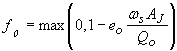
Tank structures are modelled as nodes. Suspended sediment is assumed to be well mixed throughout the tank, except for a layer of cleaner water at the surface which is discharged over the overflow. This effect may be modelled by the use of an overflow factor, ¦0. For suspended sediment:

(4) where (5) and eo is the tank efficiency associated with overflow o. The tank efficiency is defined using the US settlement efficiency or DS settlement efficiency field for the overflow link. The default tank efficiency is zero. Therefore: c0 = cJ ws is the settling velocity of the sediment (m/s) AJ is the tank area at the overflow (m2)

Numerical Techniques

A time weighted method described by Johnson and Riess (1982) is used to discretise the conservation of mass equation at each node.

(6) where 0 £ q £1 is the time-weighting parameter.

A value of q 0.5 ≥ is necessary for stability. The highest order of accuracy of the scheme is given by q = 0.5 for instance the Crank-Nicolson method (Johnson and Riess (1982)) but the solution may be oscillatory. The value q = 1 (as set in the default water quality simulation parameters file default.qsm distributed with InfoWorks ICM), for instance the implicit Euler method (Johnson and Riess (1982)) is recommended to avoid unphysical oscillations in the solution.

The cin+1 are obtained by performing a Holly-Preissmann step at the inflow from link i to node J. If the trajectory passes straight through link i during the time step, the cin+1 is related to the concentration in the node upstream of link i. This relationship, which occurs for all control structures, means that finding the solution for the nodal concentrations involves solving a matrix system. This is done using the MA48 nonsymmetric matrix solver (Harwell Subroutine Library (1993)).

Information on the Holly-Preissmann scheme is given in the Conduit Model topic.