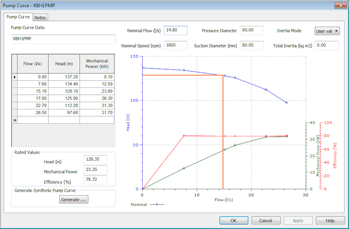
Pump Curve page

Allows viewing and editing of all the data fields shared for a Pump Curve. Details of all the fields displayed can be found in Pump Curve Data Fields.

You can display the page in two different ways:

On the Pump Grid View in the Links Grid, right click a row and choose Properties from the context menu.
On the Pump Station Property Sheet, go to the Pump Data Page, right click a row and select Pump Curve from the context menu.

The graph plots head and power from the grid, and a calculated efficiency curve. When the Nominal Flow is changed, the rated values are recalculated for that flow. See the orange line on the graph in the example picture below. The rated flows match the points where the orange line cross the various plots.

The graph is updated automatically when values in the grid or the Nominal Flow are changed. The calculated Rated Values also change.

Show me

Efficiency Curve

The efficiency curve is calculated from the Flow, Head and Mechanical Power values in the grid using the equation:

(1)

where:

P = Mechanical Power (kW)

r = Mass density of water at standard conditions (1000 kg/m3)

g = Acceleration due to gravity

H = Head

Q = Discharge through pump station

= Efficiency

Rated Values

The Rated Values on the Pump Curve Page are read only values calculated by InfoWorks WS Pro.

The rated values are calculated by interpolation of a straight line between the points of the Head, Mechanical Power and Efficiency curves either side of the nominal flow point.

Inertia

The Inertia Mode and Total Inertia fields on the Pump Curve Page are used when carrying out an InfoWorks TS (Transient System) Simulation.

Inertia describes the pump's resistance to change in momentum; the higher the inertia, the longer it will continue to rotate after shutdown.

InfoWorks WS Pro includes two in-built Inertia Modes which automatically calculate Total Inertia based on the pump's rated values using empirical relations developed by Thorley (1991). Alternatively, a user defined value may be entered.

The Total Inertia is calculated as the sum of pump inertia and motor inertia.

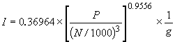
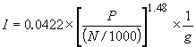
Pump inertia is calculated by InfoWorks WS Pro as:

Heavy construction (e.g. older pumps manufactured before 1970)

(2)

Light Construction (small light weight pumps)

(3)

where:

I = Inertia (kg m2)

P = Mechanical Power (kW)

N = Nominal Speed

g = Acceleration due to gravity

Motor Inertia is calculated as:

(4)

Synthetic Pump Curve

In the absence of manufacturer’s data, synthetic curves for flow, head and mechanical power can be generated.

To generate a synthetic curve

Click the Generate button on the Pump Curve Page. The Synthetic Pump Curve Generation dialog will be displayed.
In the Synthetic Pump Curve Generation dialog, select the method to be used from the following:

InfoWorks 1 point
EPANET 1 point
EPANET 3 point
WATSYS 3 point

Enter the required flow, head and nominal speed values according to the curve generation method selected.
Click OK to generate the curve.

Please Note

Generating a synthetic curve will overwrite existing values in the pump curve grid. The Nominal Flow value (and Nominal Speed if using the WATSYS 3 Point method) will also be overwritten.

The synthetic curve values may or may not agree with the actual characteristics of the pump. The user is therefore advised to use this approach only when unavoidable.

InfoWorks 1 Point Curve

A pump curve is generated using a pump head (rated head) and nominal flow specified by the user and assuming an efficiency of 80% at the pump duty point. A ten point curve is created based around the duty point using multiplying factors from tables for a typical curve.

The efficiency curve is calculated from the Flow, Head and Mechanical Power values in the grid using Equation 1 above.