Surface Washoff and Gully Pot Flushing
![]()
 Water Quality
InfoWorks ICM calculates the amount of sediment and pollutant entering the system for each subcatchment at each water quality timestep.
The water quality calculations may not take place on every hydraulic timestep. The calculation frequency depends on the value set for the QM multiplier field on the QM Parameters dialog.
The surface washoff and gully pot flushing calculations are completely independent. The following calculations take place:
- The washoff of sediment (always Sediment Fraction 1) from the surface and the resulting inflow of each attached pollutant based on their potency factors. The washoff is taken from the effective impermeability.
- The amount of each pollutant flushed from the gully pots.
Pollutant build-up
Before the start of the simulation, if you have allowed a build-up period:
- The dry weather build-up of sediment on subcatchment surfaces is calculated as described in Surface Pollutant Build-Up.
- The build-up of dissolved pollutant in gully pots is calculated as described in Gully Pot Pollutant Build-Up.
The initial Buildup Time is set on the Globals Page of the Rainfall Event Editor.
The build-up of sediment and pollutants continues during the simulation, both during storms and subsequent dry weather periods. The build-up is calculated by the same methods that are used prior to the start of the simulation.
Surface washoff
The Innovyze Surface Washoff model is based on your chosen hydraulic runoff routing model.
The software assumes that the pollutant flow at the subcatchment Drains to outlet is proportional to the quantity of pollutant dissolved or in suspension in the storm water present on the subcatchment.
The term subcatchment means the ground surface and the non-explicitly modelled network that contributes stormwater to an outlet that the subcatchment drains to in the drainage system.
InfoWorks ICM calculates the amount of:
- Sediment eroded from the surface and held in suspension in the storm water (the Total Suspended Solids). This erosion is proportional to rainfall intensity.
- Sediment washed into the drainage network using the selected runoff routing model.
- Each pollutant attached to the sediment entering the drainage network. This is also proportional to rainfall intensity.
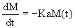
Sediment erosion
The mass of sediment eroded from the subcatchment is a function of the rainfall intensity and the mass of deposit on the ground.
|
|
where: M(t) is the mass of surface-deposit pollution (kg/ha) Ka is the erosion/dissolution factor related to rainfall intensity(1/s) |

Sediment washoff
Equation 1 determines the eroded mass per ha for the impermeable area of the subcatchment. Using your selected hydraulic runoff routing model, each runoff surface will use the same routing model and parameters as runoff to route the eroded mass. The eroded mass on a particular surface is factored by its effective impermeability as washoff should only occur from impermeable surfaces only (like road and roof).
The effective impermeability of fixed runoff volume surfaces is the runoff coefficient.
Otherwise, the effective impermeability of impervious surfaces is 1.0 and is 0.0 for pervious or unknown surfaces.
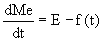
If the simulation uses the final state of another simulation to provide the initial state of the current simulation, the initial total suspended solids (TSS) outflow per surface unit is calculated from:
|
|
where: f(0) is the initial TSS outflow (kg/(s.ha)) Fm(0) is the TSS flow (kg/s) C is the proportion of subcatchment area that is impermeable Ar is the subcatchment area (ha) |

This is only relevant if the simulation used to provide the initial state included a rainfall event. The Surface Pollutant model only operates on simulations that include rainfall.
See Water Quality Simulations for more on how to use a previous simulation as the initial state for a new simulation.
Attached pollutants
The mass of each pollutant attached to the sediment washed into the system is calculated using potency factors. The potency factors depend on the rainfall intensity. These potency factors (Kpn) relate surface mass of sediment to surface mass of pollutant and are calculated using the potency factor equation:
|
|
where: IMKP is the maximum rainfall intensity over a 5-minute period in mm/hr C1, C2, C3 and C4 are coefficients |
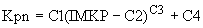
Using this equation, it is clear that the more intense the rainfall, the more important the proportion of mineral matter becomes. InfoWorks ICM assumes that the potency is constant throughout a sub-event.
The coefficients used in the potency factor equation are entered in the Surface Pollutant Editor and depend on land use, and all surface potency factors are constant throughout a given simulation.
InfoWorks ICM calculates the mass of pollutant attached to the washed off sediment using:
|
|
where: fn(t) is the pollutant flow (kg/(ha.s)) Kpn is the potency factor fm(t) is the TSS flow (kg/(ha.s)) |

Calculations for each timestep
During a simulation the following calculations are made at every timestep for surface washoff:
- Calculate the erosion rate (kg/(ha.s)). The erosion equation is
written
(5)
where:
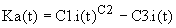
(6)
where:
Ka(t) is the rainfall erosion coefficient
i(t) is the effective rainfall in m/s
C1, C2and C3 are coefficients
On integration of the erosion equation, the erosion rate between time t and time t+dt is calculated from
(7)
- Calculate the surface buildup (kg/ha) between time tand time t+dt using the Euler approximation to
the buildup equation:

(8)
and calculate the residual surface mass (kg/ha) for use at the next time step using

(9)
- Calculate the total suspended solids (TSS) outflow per active surface
unit. The expression for TSS outflow is obtained by substituting the reservoir
equation Me = Kf(t) into the continuity equation
(10)
and integrating. For the Desbordes runoff routing model only, the TSS outflow per active surface unit is written (Equation 11). For all other runoff routing models, the washoff is routed accordingly.

where:
f(t) is the TSS flow per unit of active surface (kg/(s.ha))
K is the linear reservoir coefficient from the Desbordes runoff routing model
Me is the mass in solution per unit area (kg/ha)
M(t) is the mass of surface-deposit pollution (kg/ha)
- For the Desbordes runoff routing model only, calculate TSS outflow per subcatchment (Equation 12). For all other runoff routing models, the washoff is routed accordingly.
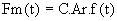
where:
C is the proportion of subcatchment area that is impermeable
Ar is the subcatchment area (ha)
calculate pollutant outflow per subcatchment:

where:
Fn(t) is the attached pollutant flow (kg/s)
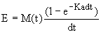
Gully pot flushing
This section describes the method for calculating the amount of dissolved pollutant removed from each gully pot at each timestep during a rainfall event.
The Gully Pot model represents the amount of dissolved pollutant washed into the system from the gully pots by runoff from the road surface.
The model uses the runoff value calculated by the hydraulic engine for Runoff Surface 1 defined in the Land Use. By convention, Runoff Surface 1 is the road surface. The runoff model used is the model you selected for hydraulic calculations in the Routing Model field on the Runoff Surface Grid Window of the Subcatchments Grid.
The underlying assumption is even mixing of the pollutant mass in the gully-pot and that resulting from surface washoff. The resulting pollutant flow depends on the inflow from the runoff module.
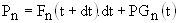
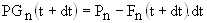
|
|
where: Pn is total pollutant mass (kg) Fn(t + dt) is dissolved pollutant inflow (kg/s) dt is timestep (s) PGn(t) is pollutant in gully (kg)
where: Q(t+dt) is runoff from road surface(m3s-1)
|
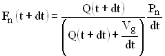
In the current model no dissolved pollutants enter the gully pot from the road surface, therefore Fn(t + dt) input to the Pn equation is always zero.