Basic 2D Hydraulic Theory

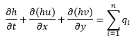
The 2D Engine used in InfoWorks ICM is based on the procedures described in Alcrudo and Mulet-Marti (2005). The shallow water equations (SWE), that is, the depth-average version of the Navier-Stokes equations, are used for the mathematical representation of the 2D flow. The SWE assume that the flow is predominantly horizontal and that the variation of the velocity over the vertical coordinate can be neglected. The conservative formulation of the SWE used in InfoWorks ICM is described below:
|
|
where: h is the water depth (m) u and v are the velocities (m/s) in the x and y directions, respectively qi is the ith net source discharge per area (m/s) ui and vi are the velocities (m/s) in the x and y directions of the ith net source discharge, respectively g is gravity acceleration (m2/s) ε is eddy viscosity (m2/s) S0,x and S0,y are the bed slopes in the x and y directions, respectively Sf,x and Sf,y are the friction slopes in the x and y directions, respectively n is the number of source discharges
|


For InfoWorks networks, turbulence contributions can be modelled using user-defined Turbulence Models (2D) which can be assigned to an entire 2D zone or specific 2D Turbulence zones. If a model is not assigned, then the effect of turbulence is considered to be included in the energy loss due to the bed resistance and modelled via the Mannings n parameter.
The conservative formulation of the SWE is essential in order to preserve the basic fundamental quantities of mass and momentum. This type of formulation allows the representation of flow discontinuities and changes between gradually and rapidly varied flow. The conservative SWE are discretised using a first-order finite volume explicit scheme. Finite volume schemes use control volumes to represent the area of interest. With finite volume methods the modelling domain is divided into geometric shapes over which the SWE are integrated to give equations in terms of fluxes through the control volume boundaries. The scheme that is used to solve the SWE is based upon the Gudunov numerical scheme, with the numerical fluxes through the boundaries of the control volumes computed using the standard Roe’s approximate Riemann solver. Finite volume methods are generally considered to have a number of advantages in terms of conservativeness, geometric flexibility and conceptual simplicity.
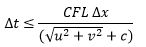
As the scheme is an explicit solution it does not require iteration to achieve stability within defined tolerances like the 1D scheme. Instead, for each element, the required timestep is calculated using the Courant-Friedrichs-Lewy condition in order to achieve stability, where the Courant-Friedrichs-Lewy condition is:
|
|
where: CFL is a dimensionless Courant number (The Timestep Stability Control set in the 2D parameters. Default=0.95) u is the velocity (m/s) in the x direction v is the velocity (m/s) in the y direction c is the flow celerity calculated as √gh (m/s) ∆t is the time step (s) ∆x is the characteristic mesh element length (m) |
The management of cell wetting and drying is performed using a threshold depth as a criteria to determine whether a cell is wet and the velocity is set to zero if the depth is below the threshold value (Depth Threshold in the 2D Parameters default=0.001m). This avoids the formation of artificially high velocities in wetting/drying areas.
InfoWorks ICM uses an unstructured mesh to represent the 2D zone and this together with the scheme used allow robust simulation of rapidly varying flows (shock capturing) as well as super-critical and transcritical flows.
2D Conduits
2D conduits (InfoWorks networks) which are connected to Connect 2D type of nodes will also be processed by the 2D engine. Details of the equations used when modelling flow in 2D conduits are included in the 2D Conduit topic.
1D-2D Linking
The 2D module of InfoWorks ICM can be linked with an InfoWorks 1D network which can be made up of conduits (urban drainage system) or river reaches. The link between 2D elements and 1D reaches is made up of lateral or in-line bank lines for 1D channels and the representation of manholes for 1D conduits. Depending on the type of manhole used to connect the 1D and 2D domains a weir equation, a head discharge or a user defined relationship is used to determine the exchange flow rate between the 1D and 2D domains. Further information can be found within the River Reach-Bank Flows and the Defining 2D Nodes topics.