About demand
One of the most important aspects of modelling a water supply system is the modelling of the demand for water from the system.
The demand for water in a given area can be divided into the following
- Domestic consumption
- Metered consumption
- Unmetered consumption
- Losses (including leakage)
- Exceptional demand (for example transfers)
Analysis of demand is usually carried out as a separate task prior to modelling the water supply system in detail. Demand analysis provides the necessary input for simulation runs (for example, demand profiles to be applied to customer points), and is also valuable information for planners, designers, and managers in the water company.
This page contains the following sections
- Demand Profiles
- Modelling of Consumption
- Losses
- Exceptional Demand
- Pressure Related Demand
- Editing Demand in InfoWorks WS
See the Demand Area Analysis topic for details of carrying out Demand Area Analysis within InfoWorks.
Demand profiles
The demand profile in an area is significantly influenced by several factors including season, day of the week, and time of day.
Daily variations
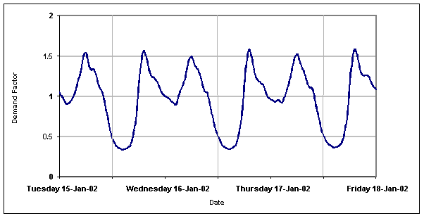
Variations of demand during the day are the most important when modelling the water supply system. The graph below shows the variations in demand over several days in a town in the UK. The daily patterns are remarkably similar, with prominent morning and evening peaks, and the same level of night consumption.
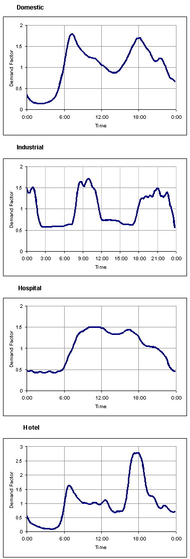
Demand in an area is made up of demand profiles of individual consumers, losses, and exceptional demand in that area. Typical profiles are often used for individual consumers in the absence of more detailed information. Some examples are shown below.
Working versus weekend days
This effect may be significant in some places and some countries. The graph below shows the variation in demand over the week for a UK town. In this example, peaks occur in the morning during the weekend.
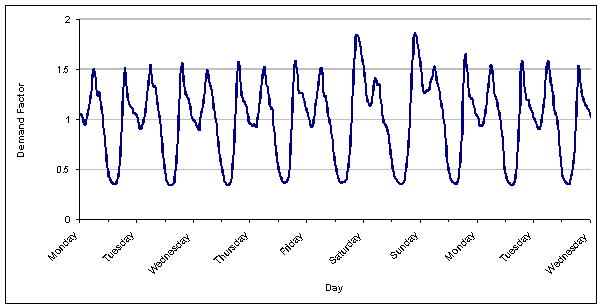
In towns with developed industry, water demand is generally higher Monday to Friday and lower during the weekend when the industrial units are closed. In tourist resorts the opposite occurs, with peak demands occurring at weekends, when the population is increased with weekend visitors.
Seasonal changes
The season has a significant effect on water consumption, both in terms of overall demand and local water use. Local circumstances are predominant. These include:
- Range of maximum and minimum temperatures
- Humidity
- Local customs
- Holiday season
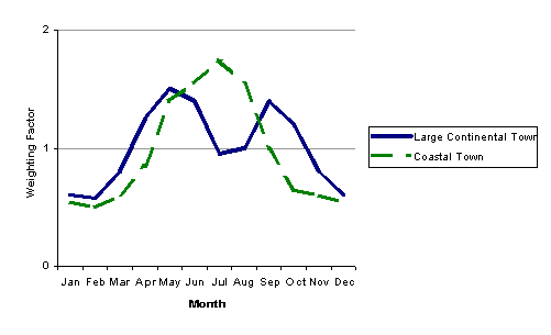
The graph below shows a comparison between a large continental town and a coastal town.
Weather Conditions
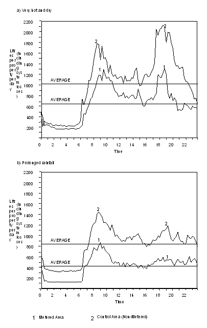
Weather conditions can be very important in some cases. The two graphs below show domestic demand patterns during metering trials in 1989 and clearly demonstrate the effects of weather conditions.
Modelling of consumption
The allocation of demand to nodes throughout the network is crucial to the eventual accuracy of the model. Any quantity of water delivered to the customer is the consumption, whether accounted for or not. Examples of customers are:
- Individual domestic properties
- Combined dwellings
- Large consumers such as hotels, hospitals, schools, farms
- Industrial estates
- Supply zones defined by the water company (small territorial units)
Customers can be classified into categories. It can be assumed that customers in the same Demand Category will use water in a similar pattern, but in different quantities. Examples of Demand Categories:
- Domestic use, individual houses
- Domestic use, large buildings
- Commercial use
- Hotels and tourism
- Hospitals, schools, universities
A true picture of daily variation is very important and no effort should be spared on this. Information from billing data, telemetry and loggers should be carefully gathered and analysed. If the data is scarce and unreliable, field tests should be organised. Demand profiles from other systems can be very misleading and should be used only for preliminary runs.
Defining a demand category
The demand profile of a customer is defined as a Demand Category using the Demand Diagram Editor. The Demand Category consists of a 24 hour water demand pattern with weighting factors for day of the week and month of the year. It is good practice to normalise the profile (i.e. to make the average value of the profile equal to one).
The water demand of one customer is defined by:
- Average consumption (usually an annual average).
- Demand category - one of those declared during model building.
The actual water demand is computed by multiplying the average consumption by the normalised Demand Category profile.
It is possible to define profiles for a Demand Category for each day of the week. Weekly and seasonal variations can be represented by the use of Daily and Monthly Coefficients, which are defined in the Demand Diagram Editor.
The water demand for each customer is calculated using the formula:
|
|
where: Km is the Monthly coefficient Kd is the Daily coefficient Kh is the time coefficient (Demand Category entry) |
See Assigning Demand to Nodesfor more detailed information on consumption at nodes.
Water demand has to be attached to the nearest ordinary or reservoir node. It cannot be attached to any other Network Object.
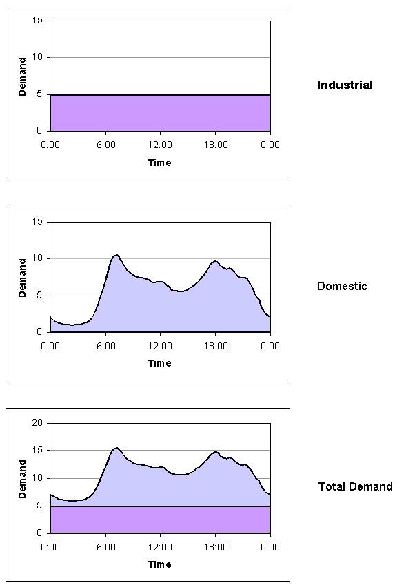
Several users may be attached to one single node. They can belong to different categories. The graph shows a simple example.
Losses
Standard practice is to increase calculated water consumption only. This is not appropriate for water supply systems, as losses behave in a quite different way to consumption. Investigations have shown that losses do not decrease during the night and increase during the day but depend mostly on the local service pressure.
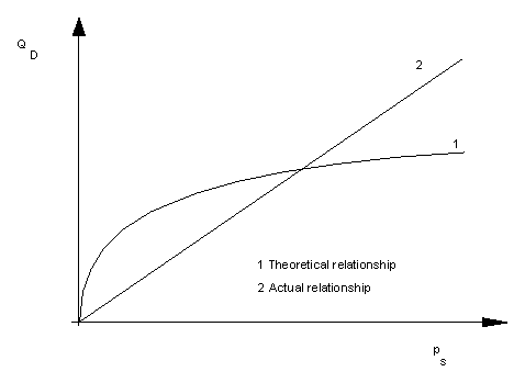
This relationship is almost linear (Leakage Control Policy and Practice (1980))and shows that losses increaseovernight.
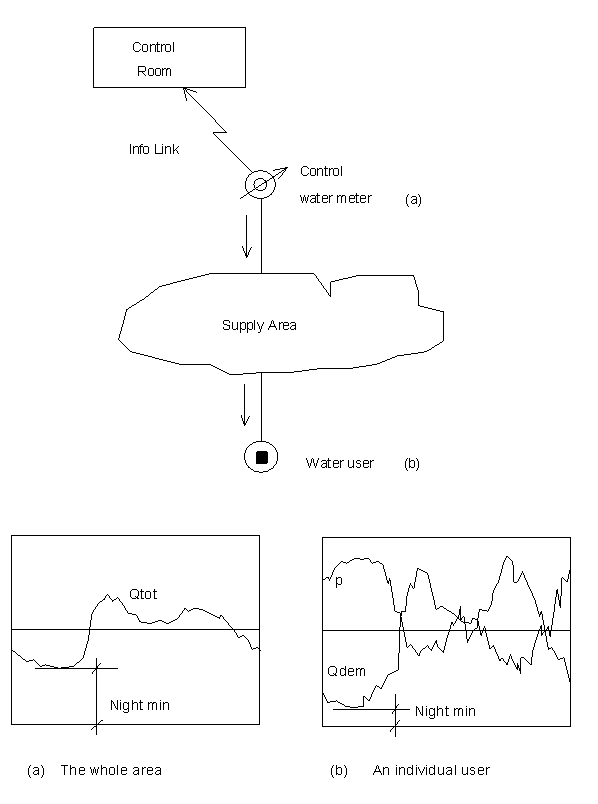
This is confirmed by studying the water use patterns for large cities. In comparing demand patterns for the whole town to those for individual users, we find that the total demand is a smoother curve - the night minimum is higher and daily peaks are lower - than individual diagrams. Losses, between 20 and 40% of total demand in many water supply systems, are time-invariant or higher at night due to increased service pressures. This tends to level the total demand over 24 hours.
Modelling of losses
InfoWorks WS Pro treats losses independently from consumption. Losses should be distributed by using all available information:
-
Assessments of unmetered demands, having made an allowance for per capita consumption
-
Analysis of minimum night flows
-
Service pressures
-
Network history
Losses should be assigned primarily to:
-
Areas of high service pressure
-
Long and/or old pipelines
-
Areas with frequent pipe bursts
InfoWorks WS Pro assumes that losses are constant during the simulation unless the user has selected the pressure-related demands and losses option. The pressure related demand method is highly hypothetical, but by careful use of reliable Live Data the user can greatly improve the model and achieve better and more realistic results.
Exceptional demand
Exceptional demand may be required for fire fighting and other emergencies, or may occur due to bursts.
The user has the option of assigning exceptional demands to one or more nodes and setting the timing, duration and intensity of such demands. An exceptional demand may be included at a node as well as, or instead of, local consumption and losses. This is particularly useful in simulating bursts in the network, to evaluate losses and to devise a defensive strategy.
The user may also use this option to simulate control policy and contingency plans to test that there are adequate reserves of water to counter possible emergencies.
For more information see Exceptional Demand and Hydrant Operation.
Pressure related demand
InfoWorks WS Pro provides an advanced option allowing you to model the influence of service pressure on demand and leakage losses. This is an advanced option and should only be used with care.
For more information, see Pressure Related Demand.
Editing demand in InfoWorks WS
For more detailed information on assigning and editing the components of demand in InfoWorks WS Pro, see the Assigning Demand to Nodes topic.
Demand diagrams
A Demand Diagram contains one or more Demand Categories that describe demand profiles for particular types of consumer. The daily demand patterns can be scaled by daily and monthly factors.
Demand Diagrams are defined and edited using the Demand Diagram Editor.
The demand diagram is an essential component of every simulation. See Simulations for more details.
Scaling demand
Demand scaling can be used to model changes in demand by applying multiplying factors to existing model demands and transfer flows assigned to nodes. This allows changes in demand (for example forecast demand increase), to be modelled without altering demand values for individual nodes.
Scale factors can be applied to demand grouped by area code and / or by demand category. Scale factors are edited using the Demand Scaling Editor.
More information about scaling demand can be found in Demand Scaling.
Every simulation can include a Demand Scaling. A Demand Scaling is included by adding it to the Schedule Hydraulic Run View. See Simulations for more details.
Demand at individual nodes
Demand can be allocated for basic nodes, reservoirs and hydrant nodes. Demand at nodes can be viewed and edited in three ways:
- Demand at individual nodes can be viewed and edited on the Node Demand Page and the Land Use Page of the Node Property Sheet.
- Demand at all nodes in the network can be viewed and edited on the Demand at Nodes Grid View.
- Wide scale adjustment of demand can be made on the Demand Adjustment View.
Static demand allocation
External Customer Point data from GIS or CSV files can be used to automatically allocate demand to nodes in the network. See Static Demand Allocation for more information.
Customer Point related demand can be updated from CSV files by using the Demand Update Wizard.
Land Use Demand Allocation
External Polygon data from GIS files can be used to automatically allocate area based demand to nodes in the network. See Allocating Land Use Demand to Nodes for more information.
Demand area analysis
InfoWorks uses information from the Network, Control, Live Data Configuration, Demand Diagram and Results files in order to carry out a Demand Analysis. The results from the analysis can be used to update Demand Diagrams and Demand at individual nodes.
See the Demand Area Analysissection for further details.